Q-Learning

The code examples and learning material I reference are based on the book: Deep Reinforcement Learning Hands-On 3rd edition.

I do not claim ownership of the original content—these notes are strictly for personal learning and reference purposes.

Q-Learning Intro

Q-Learning is similar to Value Iteration in that it seeks to learn the optimal Q-function.

However, unlike Value Iteration, which requires knowledge of the environment’s full transition probabilities, Q-Learning is model-free, which means that it learns through direct interaction with the environment.

Instead of computing the full Q-table using expected transitions, Q-Learning incrementally updates Q-values based only on the experiences it gathers during episodes (state, action, reward, next_state).

As a result, some state-action pairs may never be visited, leaving their Q-values uninitialized or unchanged. This is expected and acceptable in large or infinite state spaces.

Q-Learning Update

If you remember, the Q-iteration algorithm is as follows:

1. Initialize Q-Function table for all \((s,a)\)
2. For each \((s,a)\), update the value function: \(Q^{*}(s,a) = \mathbb{E}_{s' \sim S} \left[ r(s,a) + \gamma \max\limits_{a'}Q^{*}(s', a')\right]\)
3. Repeat step 2. until convergence.

The first expectation in step 2. implies that we are taking the expected value over the next states \(s'\). This expected value was calculated through transition probabilities of \(s \to s'\). The max part of step 2. implies that we are selecting \(a'\) that maximizes the Q-value.

For Q-Learning, we assume that we don’t know the transition probabilties. Instead, we sample from the environment of our actions

1. Initialize Q-Function table for all \((s,a)\)
2. Sample \((s, r, a, s')\) from environment
3. Update Q-Function: \(Q^{t+1}(s,a) = (1-\alpha) \times Q^{t}(s,a) + \alpha \times [ r(s,a) + \gamma \max\limits_{a'}Q^{t}(s', a')]\)
4. Repeat

As mentioned before, because we don’t have the transition probabilities, we don’t take the expecation over the next states anymore. Furthermore, we also use the current Q-function value multiplied by \(1 - \alpha\) for stability when converging our Q-Values. So the final Q-value update is a weighted average of the current reward and the reward of next_state.

Q-Learning Code (Frozen Lake)

State = int
Action = int
ValuesKey = tt.Tuple[State, Action]

class Agent:
    def __init__(self):
        self.env = gym.make(ENV_NAME)
        self.state, _ = self.env.reset()
        self.values: tt.Dict[ValuesKey] = defaultdict(float)

The initialization part is very similiar to value iteration; however, we only need our Q-Value Table for this case.

    # -- Agent() continued -- 
    def sample_env(self) -> tt.Tuple[State, Action, float, State]:
        # random actions 
        action = self.env.action_space.sample()
        cur_state = self.state
        next_state, reward, is_done, is_truncated, _ = self.env.step(action)

        if is_done or is_tr:
            self.state, _ = self.env.reset()
        else:
            self.state = new_state
        
        return old_state, action, float(reward), new_state

This is the part of sampling \((s, r, a, s')\) from environment(step 2.). One thing to note is that we selected random actions at the current state for this step and stored \((s, r, a, s')\).

    # -- Agent() continued -- 
    def best_value_and_action(self, state: State) -> tt.Tuple[float, Action]:
        best_value, best_action = None, None
        for action in range(self.env.action_space.n):
            action_value = self.values[(state,action)]
            if best_value is None or best_value < action_value:
                best_value = action_value
                best_action = action 
        
        return best_value, best_action

This is the \(\max\limits_{a'}Q^(s', a')\) part of step 3. Here we are iterating through all the actions given a state (next state, to be specific) and trying to return the max Q-Value itself and also \(a'\).

    # -- Agent() continued -- 
    def value_update(self, state: State, action: Action, reward: float, next_state: State):
        best_val, _ = self.best_value_and_action(next_state)
        new_val = reward + GAMMA * best_val
        prev_val = self.values[(state, action)]
        self.values[(state, action)] = (1 - ALPHA) * prev_val + ALPHA * new_val

Here, we are actually updating the Q-values in the table. We can see that we calculate \(Q^{t+1}(s,a) = (1-\alpha) \times Q^{t}(s,a) + \alpha \times [ r(s,a) + \gamma \max\limits_{a'}Q^{t}(s', a')]\), where we take the current reward as the input, use the ```best_val`` to get the next max Q-value, then query the current value in the Q-Value table to update our new Q-Value.

    # -- Agent() continued -- 
    def play_episode(self, env: gym.Env) -> float:
            total_reward = 0.0 
            state, _  = env.reset()
            while True:
                _, best_action = self.best_value_and_action(state)
                next_state, reward, is_done, is_truncated, _ = env.step(best_action)
                total_reward += reward
                if is_done or is_truncated:
                    break
                state = next_state
            return total_reward

We now run the entire episode and keep track of the total reward collected. Keep in mind for the Frozen Lake environment, a reward of 1 is only obtained when the goal is reached by the agent. During the episode, we can see that we query from our Q-Value table the best action to take at each state.

iter_no = 0
best_reward = 0.0
while True:
    iter_no += 1
    state, action, reward, next_state = agent.sample_env()
    agent.value_update(state, action, reward, next_state)

    test_reward = 0.0
    for _ in range(20):
        test_reward += agent.play_episode(test_env)
    test_reward /= TEST_EPISODES
    if test_reward > best_reward:
        best_reward = test_reward
    if test_reward > 0.80:
        break

In our main executable, we can see that in our loop, we first collect samples \((s, r, a, s')\) and use it to update our Q-Value table.

Then, with our Q-Value table, which is the optimal policy that we define (play episode uses best_value_and_action() to select the best action), we test whether our rewards are above our threshold of 0.8.

An important thing to note here is that our policy is deterministic here. We chose the action that returns the best Q-Value for each state. However, our environment(Frozen Lake) is stochastic. There is the slippery part that introduces randomness to the agent’s action, which is why we are taking an average over the test episodes.

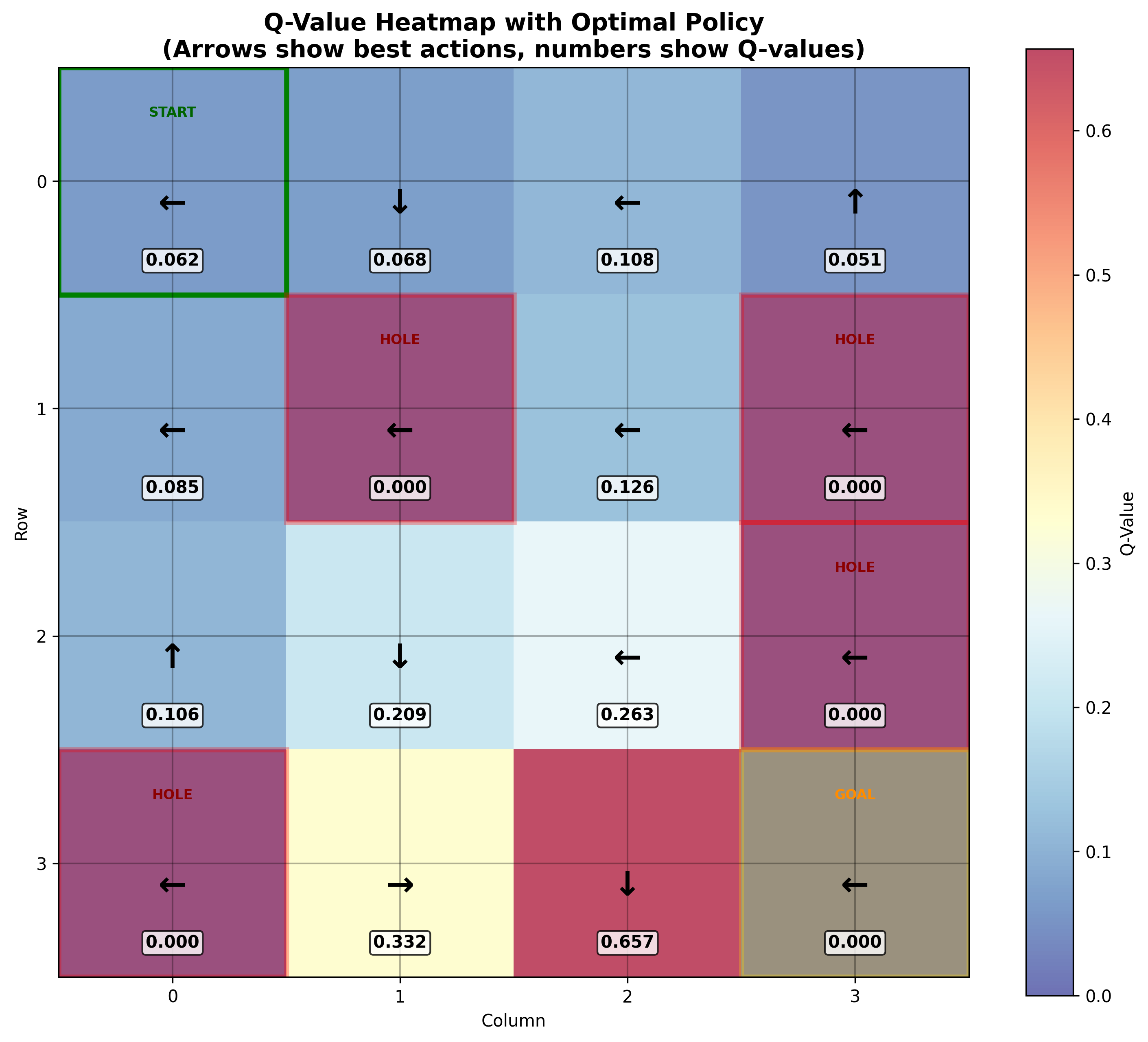
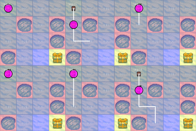
Once we execute the code and acheieve a reward over the threshold, we can actually visualize the Q-table as a heatmap based on its values. I used chatGPT for this part.

We can see that the obstacles(puddles) have a reward of 0 and that near the goal(treasure), the Q-Values are a lot higher.

Note that because the 4x4 frozen lake environment is quite small, our Q-value table is filled but it is very possible to have Q-values to be 0 for certain state-action pairs.

Thanks for reading, and next post will be on DQN!